Faster LLM Prefill With Low-Complexity Matrix Multiplication
Low-complexity matrix multiplication schemes compute the product of matrices with fewer multiplications than the textbook algorithm, at the cost of increased memory usage, limiting their practical use. Two techniques are presented to ameliorate this. First, in the neural network setting, computation of a scheme’s linear functionals can be fused with the operation preceding matrix multiplication. A way to do this in an LLM’s MLP block is described. Second, the number of writes induced by a scheme can be reduced by taking advantage of common subexpressions in its output formula. We prove the minimal number of writes induced by a scheme under this construction is seven, whereas the minimum without this construction is twelve. In ablations, common subexpressions improve performance by 2.9–3.8% and both techniques together speed up large prefills on the recent Muse Glimmer [1] and Qwen3.8 27B [2] models by 2.0–4.7% (Figure 1).
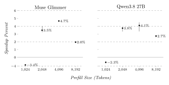
Figure 1. Batch-1 BF16 prefill wall-clock speedup over vLLM [3] on a B200 as a function of token count for two models using the low-complexity matrix multiplication techniques described here. Points are medians and error bars are interquartile ranges across ten matched fresh-process rounds, with 40 cold-L2 passes per arm per round. Code to reproduce this is is here.
1 Introduction
All low-complexity matrix multiplication schemes have the same structure. For matrices and over a ring , a low-complexity scheme requiring multiplications first computes linear combinations of the elements of each matrix,
where are linear functionals. Then, their element-wise products, , are computed and combined into the result,
A challenge in implementing low-complexity schemes is memory traffic incurred while reading and writing , as the textbook algorithm consumes directly. Recent work to address this employs clever tiling [4] or specializes for schemes which allow overlapping ’s computation with [5]. The first idea of this work is, in the neural network context, †1 to fuse computation of with the operation preceding matrix multiplication. For example, if precedes matrix multiplication, then we convert
removing much of ’s memory overhead. Fusion into can require cleverness, which §3 discusses in the context of an LLM’s MLP.
Low-complexity schemes also incur memory overhead in the reconstitution of ’s into output elements, as a naive implementation requires a write to global memory for every nonzero element of to accumulate . Fortunately, however, some low-complexity schemes’ output expressions have shared subexpressions, which can be taken advantage of to reduce memory writes.
For example, consider a chain of products,
with prefix sums
For output index , let , , and . By exchanging the summation order and telescoping,
However, because is only non-zero when , the number of memory writes needed †2 to realize this chain is how many times changes, not the number of non-zero elements of . Theorem 1 proves every chaining of a scheme induces at least seven writes, and §A provides a seven-write scheme. In contrast, the minimal number of writes induced by an unchained seven-multiplication scheme is twelve (Lemma 4).
Contributions. We imagine this work being deployed in the disaggregated prefill setting, wherein prefill and decode execute on separate GPUs [6] [7], as a scheme’s linear functionals are larger than the weight matrix they replace, reducing memory available for large decode-stage KV caches [3]. In this setting, our contributions are:
-
The first, to our knowledge, implementation of a low-complexity matrix multiplication scheme on the Blackwell architecture [8]. While work on practical low-complexity matrix multiplication has continued post-Blackwell [4] [5], older GPUs have been targeted. Roofline analysis [9] in §2.2 suggests this may be due to Blackwell being uniquely hostile to low-complexity schemes’ memory requirements (Figure 2).
-
A way to use low-complexity schemes in the neural network setting by fusing computation of a scheme’s linear functionals into the operation preceding matrix multiplication. §3 describes how to do this for the MLP block of an LLM, where fusion is complicated by nonlinearity.
-
Chaining, a method for reducing memory traffic induced by a scheme during reconstitution of its products into output elements, together with a lower bound. Every chaining of every seven-multiplication scheme induces at least seven writes (Theorem 1). The scheme of §A attains this.
2 Background & Related Work
2.1 Low-Complexity Schemes
The shared structure of low-complexity schemes is due to -multiplication schemes corresponding to rank- decompositions of the matrix multiplication tensor [10] [11]. Recent years have witnessed considerable progress on techniques for finding low-rank decompositions of this tensor [12] [13]. This can aid implementations; for example, some schemes require fewer additions to compute and our optimal scheme admitting a seven-write chaining was discovered via search over thousands of rank-seven decompositions of the matrix multiplication tensor.
An scheme can be lifted to compute the product of matrices by interpreting them as matrices over the ring of matrices. We’ll prove this for the case, but the main idea is easily translated to arbitrary and non-square matrices with dimensions divisible by .
For matrices and any length- vector , write and to denote the first and second halves of and likewise divide into four submatrices.
After mechanically expanding the matrix product applied to an arbitrary input,
it is clear the product of a reinterpretation of as matrices of matrices agrees with their standard product on all inputs, so is the same linear function, i.e. is the same matrix. A scheme valid over arbitrary rings gives an alternative way to compute the formula for the re-interpreted matrix product, and therefore an alternative way to compute , as matrices are themselves a ring with matrix addition and multiplication.
2.2 Low-Complexity Scheme Implementations
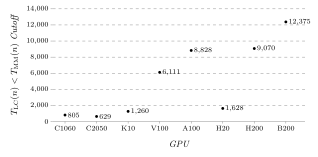
Figure 2. Predicted value of for which a , seven-multiplication scheme that does not fuse linear-functional computation multiplies matrices faster than the textbook algorithm. C1060, C2050, and K10 GPUs consider four-byte floats, as two-byte floats are unsupported; the remaining GPUs consider two-byte floats.
As modern GPUs have increased the ratio of floating-point operations per second to memory bandwidth, so too has the difficulty of implementing low-complexity matrix multiplication schemes; hence a long history of efforts beginning with Li et al.’s 2011 work on the NVIDIA Tesla C1060 [14], followed in 2013 by Lai et al. on NVIDIA Fermi and Kepler GPUs [15], in 2020 and 2022 by Huang et al. and AlphaTensor on the NVIDIA V100 [16] [12], and in 2026 by SubCuber [5] and FalconGEMM [4] on the NVIDIA H200, A100 and H20 GPUs.
To explain this growing difficulty, let be a GPU’s floating-point operations per second and be its memory bandwidth in bytes per second. It is typical [9] to model the time required to multiply two matrices of two-byte floating-point numbers with the textbook algorithm as
where the maximum of compute and memory time is taken as efficient implementations overlap memory and compute. We omit the memory cost incurred writing the result to memory for simplicity, though, as discussed, including it would further benefit the textbook algorithm for comparison purposes.
A standard implementation of an -multiplication scheme will incur
bytes of memory traffic while computing its linear functionals, for a total time cost of
In the compute-bound regime, solving for when a low-complexity scheme is predicted to be faster than a textbook matrix multiply yields
Plotting this cutoff for a seven-multiplication scheme and each mentioned GPU (Figure 2) motivates our decision to fuse linear functional computation.
2.2.1 FalconGEMM
Our low-complexity matrix multiplication implementation builds on several great insights from the work of Zhu et al. on FalconGEMM [4].
First, for the purposes of computing linear functional outputs, Zhu et al. notice that, for an scheme, each tile of linear functional output depends only on corresponding tiles in the linear functional input. For example, when the illustration below shows how a CTA can compute a tile of every linear functional’s output when it owns four tiles of the input.
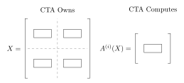
This is possible because the operations in linear functional computation, matrix addition and scalar multiplication, happen elementwise. We make use of this observation in designing our fused kernels.
Second, like FalconGEMM, we assign each CTA to a distinct tile of the output, which allows overlapping writing to global memory with computing . †3 However, as Zhu et al. note, this increases the amount of computation per CTA, thereby increasing the opportunity cost of underfull waves. For example, the illustration below shows a case where, for a per-CTA tile size and a GPU capable of executing a grid of CTAs, the third wave of execution is underfull, leaving one CTA worth of computation on the table.
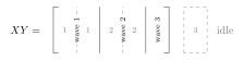
FalconGEMM resolves this via somewhat-involved scheduling whereby computation of s is divided up amongst the GPU’s processors according to a schedule which maximizes the frequency with which a single processor owns . So, in the example above, computation of the third wave’s tile would be divided among two processors, one of which computed and the other the rest. This improves utilization at the cost of cross-CTA coordination, as ’s accumulation into global memory must be ordered with respect to the previous product’s writes to avoid overwriting.
Perhaps due to a skill issue (FalconGEMM is not open source at the time of writing), or perhaps due to particularities of the GPU (B200 versus A100 and H20), we were unable to implement this scheduling in a way that improved performance. Instead, we achieve a similar effect by varying per-CTA tile sizes in later waves. For example, we might assign CTAs in wave three tiles.
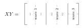
This improves utilization at the potential cost of tensor core utilization in smaller tiles in late waves.
3 Linear Functional Fusion
Consider the MLP in the Muse Glimmer model which, on an input , computes
vLLM spends roughly two-thirds of 4096-token prefill execution time here, hence interest in speeding it up. This section transforms the MLP into
where the and matrix multiplications are, naturally, performed with low-complexity schemes.
For the remainder of this section, fix a low-complexity scheme and suppose are square matrices. The scheme thus views as a matrix over ,
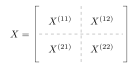
In turn, each linear functional is of the form
Recall that, in the neural network setting, can be precomputed, as is a weight matrix, so we consider only .
The RMSNorm kernel in vLLM assigns each CTA a row of , which is incompatible with CTAs being responsible for a tile of , as row of is a function of rows and of ,
Hence, to compute , CTA is assigned rows and of , then takes the requisite linear combinations of , , , and , which it has just computed, to compute the th row of each linear functional.
The kernel assigns each CTA four tiles of , one per low-complexity quadrant,
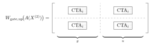
Each of these tiles is computed per the low-complexity scheme, then, per the function (), are folded together by the CTA.
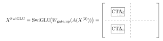
This leaves each CTA with two tiles of output, not enough to compute a tile of . Suppose, however, the width of ’s tile is columns, and consider a permutation, , of the columns of the output which moves odd-numbered width- groups of columns to the right half of the matrix.
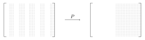
Each CTA owns four tiles of a version of the ’s output with applied.
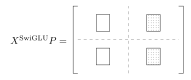
Hence, without any data movement, each CTA in our kernel actually computes a tile of , and is fed in as the second argument to the low-complexity computation, compensating for the permutation and yielding , as expected.
4 Optimal Schemes, Chains
The seven-write chaining of a scheme used by our implementation (§A) is optimal; i.e. there is no six-write chaining of a seven-multiplication scheme.
An -product chain is a scaling and reordering of a subset of a scheme’s products
where are nonzero, along with a write schedule which indicates that prefix sum
should be accumulated (written) into output after being scaled by . The total number of writes induced by a chain is therefore the number of non-zero elements in its write schedule, A chaining of a scheme is a partitioning of its products into chains whose write schedules collectively compute the scheme.
Theorem 1. The minimum number of writes induced by a chaining of a seven-multiplication scheme over is seven.
Lemma 1. The coefficients on products in a seven-multiplication scheme for matrix multiplication are non-proportional; i.e. if then there is no non-zero scalar such that .
Proof. Per deGroote’s 1978 proof [18], all seven-multiplication schemes are equivalent to Strassen’s [19] modulo sandwich, scaling, and permutation symmetries. In particular, a scheme with decomposition is related via a sandwich symmetry to one with decomposition if
for invertible matrices ; summands with nonzero satisfying are related by a scaling symmetry to ; and schemes are related via a permutation symmetry if a reordering of one’s summands yields the other. Applied to the coefficients of a scheme, this yields
where are Strassen’s coefficients, is a non-zero scalar, is an invertible linear map, and is a permutation.
By inspection, the usual Strassen coefficients,
are non-proportional. So, towards a contradiction, if for some and non-zero scalar in a seven-multiplication scheme, then
but this contradicts the non-proportionality of Strassen’s coefficients. Hence, and are non-proportional. ◻
Lemma 2. The products of a seven-multiplication scheme for matrix multiplication are linearly independent.
Proof. If, modulo reordering and towards a contradiction,
then there is a rank-six decomposition of the matrix multiplication tensor,
contradicting Winograd’s 1971 result [20] that matrix multiplication requires seven multiplications. ◻
Lemma 3. Let
for , and let be . The number of writes at step of an -product chain is
Proof. A chain’s contribution to the output is
Per Lemma 2 and because the chaining correctly computes the scheme, the coefficient on must be , hence so and therefore and . ◻
Proof of Theorem 1. In any length- chain for a seven-multiplication scheme, as is definitionally zero, by Lemma 3
so as being zero would allow to be removed from the scheme, yielding a six-multiplication scheme, contradicting the minimality of seven-multiplication schemes [20]. Moreover, for
is zero only if
so per Lemma 1 . Hence, a length- chain induces at least writes. The sum of lengths of chains in a chaining of a scheme is the number of products in the scheme, so every chaining induces at least seven writes. The seven-write chaining of §A attains this lower bound. ◻
5 Evaluation
Having established our kernels can speed up large prefills (Figure 1), our evaluations consider three questions: (1) Do the different floating-point numerics of low-complexity schemes degrade model performance? (2) Does reducing the number of writes, à la chaining, speed up our implementation? (3) Are prefill speedups due to our MLP fusion design or low-complexity schemes? All three resolve favorably for low-complexity schemes.
All these experiments ran on an NVIDIA B200 (180 GB HBM), vLLM commit 99a10304d, PyTorch 2.13.0/CUDA 13.0, and Triton 3.7.1. We used BF16 Muse Glimmer 30B and Qwen3.8 27B checkpoints. Timings used fresh-process runs, a clear L2 cache, and LLM prefill measurements used batch size one.
5.1 Low-Complexity Numerics
Following the evaluation used by Atom [21], we measure perplexity on the WikiText-2 test set [22]. We use a context length of 2,048 and BF16 weights and activations. Table 1 compares the stock implementation and the mean of six independent runs using our kernels. Our overall effect on perplexity is less than three hundredths of one percent for both models.
| Model | Stock | Ours | Relative change |
|---|---|---|---|
| Muse Glimmer | 8.182328 | 8.182803 | |
| Qwen | 9.293222 | 9.295323 |
Token-level perplexity on WikiText-2. “Ours” is the mean of six independent runs. 95% confidence intervals for the relative change are for Muse Glimmer and for Qwen.
Following FlashAttention-3’s operator-level analysis [23], we also compare the outputs of the conventional and low-complexity MLP computations. At a prefill length of 2,048, the relative Frobenius error is after the gate and up projections and after the down projection.
To determine how these local differences propagate through the model, we evaluate stock vLLM versus our kernels on HellaSwag [24], ARC-Challenge [25], and the high-school mathematics subset of MMLU [26]. We report normalized accuracy for HellaSwag and ARC-Challenge (as is conventional) and accuracy for MMLU.
| Model | Kernel | HellaSwag | ARC-Challenge | MMLU HS Math |
|---|---|---|---|---|
| Muse Glimmer | Stock | 82.72 | 62.37 | 51.48 |
| Ours | 82.77 | 62.80 | 52.22 | |
| Qwen | Stock | 82.86 | 58.79 | 61.48 |
| Ours | 82.89 | 58.62 | 61.48 |
Task accuracy in percent. HellaSwag and ARC-Challenge use normalized accuracy.
Across the six model-task pairs, the change ranges from to percentage points, and every difference is smaller than the corresponding per-arm standard error. Taken together, operator errors, perplexity measurements, and downstream evaluations suggest our kernels have little impact on model behavior.
5.2 Chaining Ablation
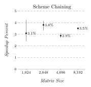
Figure 3. Speedup from scheme chaining for square BF16 matrix multiplications versus unchained kernels with a clear L2 cache. Points are medians of ten paired round-level speedups; lines show the interquartile range.
Figure 3 ablates scheme chaining. The unchained comparison was independently optimized at each matrix size. †4 Even against this tuned control, chaining improves performance by – across the tested sizes.
5.3 Low-Complexity Ablation
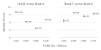
Figure 4. Batch-1 BF16 Muse Glimmer prefill wall-clock comparisons on a B200. (Left) Stock vLLM is faster than the textbook (rank-eight) scheme on all measured sizes. (Right) A rank-seven scheme (the seven-write appendix) beats the textbook one at all measured sizes. Points are medians and error bars are interquartile ranges across ten matched fresh-process three-arm rounds, with 40 cold-L2 passes per arm per round.
An interpretation of the textbook matrix-multiplication algorithm as a rank-eight scheme admits, structurally, the same fusion as our MLP-replacement kernels but without reduced multiplications. Figure 4 compares the performance of this reinterpretation of the textbook scheme with stock vLLM and our rank-seven scheme at various prefill sizes. Despite tuning the rank-eight kernel to achieve near-identical active-warp percentages and using chaining †5, the rank-seven scheme outperforms the textbook one at all measured sizes. It seems prefill performance increases are due to low-complexity schemes, not a side-effect of our fusion design.
6 Limitations & Future Work
One cause of increased memory usage in low-complexity schemes remains unaddressed by this work: Under a seven-multiplication scheme, linear functionals are 75% larger than the weight matrices they replace, as, in general, an -multiplication scheme’s linear functionals have size . For Muse Glimmer and Qwen3.8 27B storing instead of weight matrices increases storage by 52.22% and 46.2%, respectively. In the disaggregated prefill setting we consider here, this is not problematic for the GPU, prefill sizes, or models. We leave balancing the tradeoff between storage, transformation cost, and throughput in the decode setting to future work.
We leave one possible direction for resolving this. As is a redundant encoding of , one might search for schemes which allow exploitation of shared sub-terms in linear functionals to partially materialize , then fully materialize on demand. The scheme in §A, for example, admits a compressed representation in this way. Given and one can construct the remaining linear functional outputs via
Hence, with no storage penalty, one could store and and compute the remaining values online.
7 Conclusion
We believe the common belief that low-complexity matrix multiplication schemes are impractical for practical matrix sizes may be false. While, in isolation, roofline analysis indicates memory overhead incurred computing linear functionals is unfavorable on modern GPUs (§2.2), in practice, much contemporary matrix multiplication occurs in the neural network setting where linear functional computation can be fused with the operation preceding matrix multiplication (§3). Moreover, a novel chaining technique (§4) can reduce the memory overhead incurred in reconstituting a scheme’s products into its output. Our implementation of these techniques speeds up large prefills on the recent Muse Glimmer [1] and Qwen3.8 27B [2] models (Figure 1).
Appendix
A scheme with a seven-write chaining
The scheme’s linear functionals are
and the unchained reconstruction is
We partition these products into the three chains
Let these chains’ prefix-sums be , , and respectively. Our matrix multiplication kernel uses a depth-two pipeline, so prefix-sums are accumulated into the stage’s two TMEM accumulators. The execution schedule is:
which computes
Notice how, at any step, at most two prefix-sums are resident; hence the prefix-sums can be stored in a standard, pipelined, depth-two matrix multiplication kernel’s TMEM accumulators, incurring no additional memory traffic.
This chaining was discovered by a somewhat interesting but out-of-scope exhaustive search over ternary seven-multiplication schemes. We were later able to prove its minimality over all schemes via Theorem 1.
B Minimum writes induced by an unchained, seven-multiplication scheme
The number of writes induced by an unchained scheme is its number of non-zero elements.
Lemma 4. The minimum number of non-zero elements in a seven-multiplication scheme is twelve; i.e.
Proof. Per deGroote’s 1978 proof [18], all seven-multiplication schemes are equivalent to Strassen’s modulo sandwich, scaling, and permutation symmetries. For Strassen’s coefficients (see Lemma 1), has rank two and have rank one. Moreover, writing
the and occupy three distinct one-dimensional subspaces of , each twice. Permutation and scaling symmetries preserve this structure.
Sandwich symmetries left- and right-multiply s by invertible linear maps, preserving matrix rank and mapping distinct one-dimensional subspaces to distinct one-dimensional subspaces. Hence, in every seven-multiplication scheme, one has rank two and the remaining six can be written such that the and occupy three distinct one-dimensional subspaces, each twice.
At most two distinct one-dimensional subspaces of contain a vector with only one non-zero element. So at least one of the three distinct one-dimensional subspaces occupied by the and has two non-zero elements, so
As
the six rank-one coefficients contain at least
non-zero elements. The remaining coefficient has rank two, hence contains at least two non-zero elements, so
Strassen’s coefficients have twelve non-zero elements, so the bound is tight. ◻ is a fixed weight matrix, so can be computed offline.
values can be accumulated in Blackwell TMEM, thus do not incur global writes. FalconGEMM keeps output tiles on-chip, but on newer NVIDIA GPUs this design allows overlapping using the TMA reduce-add store operation [17]. Before discovering the chaining design, we extensively iterated on and optimized an unchained kernel, so we believe this is a fair comparison. The textbook algorithm for matrix multiplication admits a four-write chaining.References
-
Muse Glimmer-30B. Meta Superintelligence Lab. 2026.
-
Qwen3.8-27B. Qwen Team. 2026.
-
Efficient Memory Management for Large Language Model Serving with PagedAttention. Kwon, Woosuk and Li, Zhuohan and Zhuang, Siyuan and Sheng, Ying and Zheng, Lianmin and Yu, Cody Hao and Gonzalez, Joseph E. and Zhang, Hao and Stoica, Ion. 2023.
-
FalconGEMM: Surpassing Hardware Peaks with Lower-Complexity Matrix Multiplication. Honglin Zhu and Jiaping Cao and Jiang Shao and Siyuan Feng and Qian Qiu and Peng Chen and Xu Zhang and Yixian Zhou and Man Lung Yiu and Guang Ji and Minwen Deng and Jintao Meng and Wenxi Zhu. 2026.
-
Compiling Strassen-like Matrix Multiplication Algorithms to Fast CUDA Kernels. Abhinav Jangda. 2026.
-
Splitwise: Efficient Generative LLM Inference Using Phase Splitting. Patel, Pratyush and Choukse, Esha and Zhang, Chaojie and Shah, Aashaka and Goiri, 'I\ nigo and Maleki, Saeed and Bianchini, Ricardo. 2024.
-
DistServe: Disaggregating Prefill and Decoding for Goodput-optimized Large Language Model Serving. Zhong, Yinmin and Liu, Shengyu and Chen, Junda and Hu, Jianbo and Zhu, Yibo and Liu, Xuanzhe and Jin, Xin and Zhang, Hao. 2024.
-
NVIDIA Blackwell Architecture Technical Brief. NVIDIA Corporation. 2024.
-
Roofline: An Insightful Visual Performance Model for Multicore Architectures. Williams, Samuel and Waterman, Andrew and Patterson, David. 2009.
-
On Schemes for the Computation of Products and the Inverse Matrix. Pan, Victor Ya.. 1972.
-
On the Optimal Evaluation of a Set of Bilinear Forms. Brockett, Roger W. and Dobkin, David P.. 1973.
-
Discovering Faster Matrix Multiplication Algorithms with Reinforcement Learning. Alhussein Fawzi and Matej Balog and Aja Huang and Thomas Hubert and Bernardino Romera-Paredes and Mohammadamin Barekatain and Alexander Novikov and Francisco J. R. Ruiz and Julian Schrittwieser and Grzegorz Swirszcz and David Silver and Demis Hassabis and Pushmeet Kohli. 2022.
-
Flip Graphs for Matrix Multiplication. Kauers, Manuel and Moosbauer, Jakob. 2023.
-
Strassen's Matrix Multiplication on GPUs. Junjie Li and Sanjay Ranka and Sartaj Sahni. 2011.
-
Accelerating Strassen-Winograd's Matrix Multiplication Algorithm on GPUs. Pai-Wei Lai and Humayun Arafat and Venmugil Elango and Ponnuswamy Sadayappan. 2013.
-
Strassen's Algorithm Reloaded on GPUs. Jianyu Huang and Chenhan D. Yu and Robert A. van de Geijn. 2020.
-
CUTLASS Tutorial: Mastering the NVIDIA Tensor Memory Accelerator (TMA). Colfax Research. 2024.
-
On Varieties of Optimal Algorithms for the Computation of Bilinear Mappings. II. Optimal Algorithms for -Matrix Multiplication. de Groote, Hans F.. 1978.
-
Gaussian Elimination is Not Optimal. Volker Strassen. 1969.
-
On Multiplication of Matrices. Shmuel Winograd. 1971.
-
Atom: Low-Bit Quantization for Efficient and Accurate LLM Serving. Zhao, Yilong and Lin, Chien-Yu and Zhu, Kan and Ye, Zihao and Chen, Lequn and Zheng, Size and Ceze, Luis and Krishnamurthy, Arvind and Chen, Tianqi and Kasikci, Baris. 2024.
-
Pointer Sentinel Mixture Models. Merity, Stephen and Xiong, Caiming and Bradbury, James and Socher, Richard. 2017.
-
FlashAttention-3: Fast and Accurate Attention with Asynchrony and Low-Precision. Shah, Jay and Bikshandi, Ganesh and Zhang, Ying and Thakkar, Vijay and Ramani, Pradeep and Dao, Tri. 2024.
-
HellaSwag: Can a Machine Really Finish Your Sentence?. Zellers, Rowan and Holtzman, Ari and Bisk, Yonatan and Farhadi, Ali and Choi, Yejin. 2019.
-
Think You Have Solved Question Answering? Try ARC, the AI2 Reasoning Challenge. Clark, Peter and Cowhey, Isaac and Etzioni, Oren and Khot, Tushar and Sabharwal, Ashish and Schoenick, Carissa and Tafjord, Oyvind. 2018.
-
Measuring Massive Multitask Language Understanding. Hendrycks, Dan and Burns, Collin and Basart, Steven and Zou, Andy and Mazeika, Mantas and Song, Dawn and Steinhardt, Jacob. 2021.
Thanks to John for advocating for the B200 access which made this possible. Also to Alayt, Anagha, Ashvin, Danny, Esme, Federico, Grace, Moses, Natalie, Nick, Noah, Pete, Quan, Sophia, Tejas, Tonya, and Zeno, for countless interesting conversations.