Tiny -CROWN
Neural networks, for example image classifiers, are often vulnerable to attacks where small, sub-perceptual changes to the input cause misclassification.
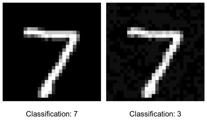
Figure 1. Left: an image classified as 7 by the neural network
from tinygrad's quick-start MNIST
example. Right: a
small perturbation changes its
classification to 3.
Informally, given an input to a neural network , the verification problem is to prove that for any that is a bounded perturbation of , . Successful proofs can rule out attacks like the one above.
The current state of the art is an algorithm called -CROWN, an implementation of which has won the International Verification of Neural Networks Competition for the past five years. I think -CROWN is a lovely algorithm in an important research area where progress is unlikely in my lifetime.
I implemented -CROWN for a deep-learning library called tinygrad and this blog post is about how it works. This is for the most part a synthesis of these three papers, my very modest contribution being a description of how the algorithm handles shape changes (reshape/flatten/permute) which does not appear in existing descriptions.
Background
is a bounded perturbation of if it is an element of an -ball of radius centered at , denoted :
where is 's -norm,
A convenient fact is that there is a closed-form solution to the minimum of any linear (or affine) function over an ball (Hölder's inequality):
where denotes the dot product of vectors and , and is the dual norm of , defined by
In image classification, for an image , a neural network typically outputs an -dimensional vector and 's classification is said to be the index in with the largest value. Thus, for the example in Figure 1, proving no bounded perturbation of an image gets classified as 3 is equivalent to checking that In turn, a common approach to neural network verification (and the one taken by -CROWN) is to compute affine bounds on the output of , then use Hölder's inequality to minimize over . If the minimum is , then no images in a bounded perturbation of will be classified as 3.
-CROWN on Graphs
Many deep-learning libraries represent neural networks as graphs where edges correspond to data and vertices to differentiable operations. For example, might be represented as

To implement -CROWN on a graph, we need a way to compute
bounds on the output of each operator given bounds on its input, then
bounds on the output of the network can be propagated through the
graph and written in terms of the network's input. For example, for
the + operator above, if
are affine lower bounds on and , then
is a lower bound on .
Handling ReLU
Nonlinear functions like ReLU are more challenging to bound. -CROWN uses linear over/under-approximations.

Figure 3. The dashed lines are linear bounds on a ReLU over the interval .
First, Hölder's inequality is used to compute concrete bounds and on the ReLU's input. Then, when (i.e. the ReLU is nonlinear), for some , letting denote ReLU, the following equations bound it:
Notice how any value of between zero and one gives a lower bound when . Thus, towards choosing a good value for , notice that the ReLU bounds, the function bounds, and Hölder's inequality are all computed using differentiable operations. In fact, in general, all the equations for bound propagation in -CROWN are differentiable. In turn, given bounds on a neural network's output in terms of different ReLU's values, we can use gradient descent to find values that tighten them. I think this is cool!
-CROWN
In Figure 3, if or , then setting to 1 or 0 makes the ReLU bounds exact; ReLU's with this property are called stable. If we can compute bounds on conditional on a ReLU being stable, we could consider both cases and merge them. For example, if were lower and upper bounds on a ReLU when , and were bounds when , then
are overall bounds on the ReLU. This is the idea behind -CROWN. To propagate bounds on to ,
subject to constraints , we let be positive if satisfies and negative otherwise. For example, in the case where the constraint enforces , we have . Then, if
by Lagrangian relaxation and weak duality,
where . To find a value for that gives a tight bound we can, once again, use gradient descent. Notice that the term can be removed by recursively getting bounds on in terms of . Bounds for the and cases can be merged to get overall bounds on the ReLU as described above. Finding upper bounds is a variant of the same procedure as .
tinygrad
tinygrad is a popular deep-learning library with lazy evaluation and a
small set of UOps to which tensor operations are lowered before
being run. Because tinygrad is lazy, tensors are represented as a
graph that computes their value on demand, making accessing a
computation's graph straightforward. Furthermore, tinygrad's small set
of UOps means bound propagation only needs to be implemented for
this small operation set to support complex networks. These properties
make tinygrad amenable to an implementation of -CROWN.
However, tinygrad's UOps are distinct from the operations described
in previous work on -CROWN. For example, whereas
-CROWN considers matrix multiply a primitive operation,
tinygrad compiles matrix multiply to a series of low-level shape
changes. Specifically, for , tinygrad
computes via:
While available implementation of -CROWN handle shape changes, published descriptions of the algorithm don't, instead describing how to compute bounds on in terms of vectors and matrices :
When the input to the network is not a vector (for example, an image with shape ), the matrix multiply above is no longer semantically valid. Thus, beyond an -CROWN implementation for tinygrad, this blog's small contribution in the following section is a description of how to compute -CROWN bounds for arbitrarily shaped inputs subject to arbitrary shape changes. The method is semantically identical to the one used by -CROWN's existing PyTorch implementation.
Handling Shape Changes
To handle high-rank tensors and shape changes in tinygrad, bounds on the network are written in terms of tensor contractions.
For with shape and with shape the tensor contraction of and is written,
Intuitively, can be thought of as describing the linear combination of elements of that make up index in the result.
To handle shape changes like permute, expand, reshape, and
shrink notice that all of these can be described by a function
mapping an index in the resulting tensor to an index in
the original tensor. Applying a shape change to the bounds is thus
equivalent to moving the linear combination of elements of used to
compute index to index , i.e. applying the shape change to
's leading dimensions. I think this is quite
elegant and was happy to figure it out.
The code is available here.
Thanks to Dhruv for working on this with me, Michael Everett for a great class, and Nick and Noah for interesting conversations.