Cellular Automata Surviving Steps
Recent work by Wolfram composes pairs of elementary cellular automata to ``survive steps'' — maintaining at least one cell for steps before transitioning to exclusively . This formalizes and analyzes the problem of surviving steps. We develop techniques for analysis of inhomogeneous cellular automata based on Boolean satisfiability and binary decision diagrams that classify 99% (of 32,640) pairs of elementary automata as able to solve Survive--Steps for an infinite, or finite, number of . We measure the performance impact of various heuristics on our SAT-based analysis and find, while learned clauses slow down the solver, variable selection heuristics are critical for performance.
1 Introduction
Recent work by Wolfram [1] has synthesized inhomogeneous cellular automata [2] from pairs of elementary rules using an evolutionary algorithm. The main focus is automata that survive steps -- having a cell in the first states and thereafter exclusively cells -- henceforth the Survive--Steps problem (see also [3], [4]).
This post empirically and analytically analyzes the Survive--Steps problem with ideas from formal methods. We develop a novel reduction of inhomogeneous cellular automata to Boolean satisfiability. Then, using a SAT solver, binary decision diagrams, and purely analytical methods, classify 99% of pairs of elementary rules as able to survive steps for an infinite, or finite, number of . We also comprehensively solve, or prove the unsolvability of, Survive--Steps for for every pair of elementary rules with our SAT-based synthesis technique, finding there is rich structure to what pairs of rules can survive steps.
1.1 Example
Consider if elementary cellular automata rule 18 and 82 can be composed to survive steps. An illustration of the input/output pairs for the automata is given below.


Elementary cellular automata are functions that take three inputs and produce one output.  being drawn in rule 18's box means on input
  rule 18 will output . As the illustration shows, for the most part, rules 18 and 82 are the same, only differing on input . This will give them interesting behavior when surviving steps.
Elementary cellular automata "grow" from an initial state. To determine a cell's value in the next state, the value of the cell to the left, the cell's current value, and the value of the cell to the right are input to the automaton's function. The automata in this post are grown on finite-width states, so cells on the edge "wrap around": The cell to the left of the leftmost cell is the rightmost cell and the cell to the right of the rightmost cell is the leftmost cell.
For example, on the left side of the illustration below rule 18 is grown from an initial state with three cells and two cells. The second row of the drawing is the second state of the automaton. From left to right, the value of each cell in the second state is determined by the input/output pairs  ,
,  ,
,  , , and
  .
.

With inhomogeneous elementary cellular automata, we can choose which rule determines the value of each cell. For example, on the right-hand side of the illustration above rule 82 is chosen to determine the value of the 4th cell in the second state, changing its value to . In the illustration, patterns disambiguate which rule determines the value of each cell.
Two rules can survive steps if, starting from an initial state with exactly one cell, there is a choice of what rule to use where, such that there is at least one cell in the first states and only cells thereafter. For example, in the illustration below, rules 18 and 82 are composed to survive steps.

Notice for values of , rules 18 and 82 cannot survive steps, as no matter what automaton is used where, the first three states will be the same. It is only in the third state, when, due to wrapping, the pattern appears. Because the rules differ on this input, rule 82 can be chosen, causing the automaton to "die".
The question this post asks is, for an arbitrary pair of rules, is there an infinite number of for which Survive--Steps is solvable? For rules 18 and 82, we'll now show the answer is infinite. Consider the choice of rules in the illustration below and notice how the final state has a single cell.

From this and our previous solution to Survive--Steps, we know how to (1) start from a state with a single cell and return to a state with a single cell after steps, and (2) start from a state with a single cell and "die" after steps. Even though the start/end position of the cell in the drawing above is different, because states wrap at the edges, we can "rotate" a choice of what rule to use where to line up cells (Lemma 2 will formalize this). Thus, we can compose our automata to survive steps for any expressible as , an infinite number of . For example, for the illustration below gives a solution to Survive--Steps.

Throughout this post, we'll formalize and automate this technique (c.f. §6.3) and several others for exactly characterizing the set of for which Survive--Steps is solvable on a width- board. New ideas will be required to identify when Survive--Steps is unsolvable and to automate the synthesis of the examples in this section.
1.2 Organization
In §3, we give a formalization of inhomogeneous elementary cellular automata, Survive--Steps, and some basic lemmas about their behavior. Using this formalization, we reduce the Survive--Steps problem to Boolean satisfiability in §4. This equips us with powerful analysis tools from formal methods: SAT solvers and binary decision diagrams. These are many orders of magnitude faster than Wolfram's evolutionary synthesis technique [1] (though, we emphasize, the focus of that work is not performance). For example, even having implemented a reasonably efficient version of Wolfram's technique in C (random-guessing.c in the associated code §8), it would run for hours and fail to synthesize a solution to Survive--Steps for most rule tuples, whereas the SAT solver takes seconds. While the focus of our work is analysis, not synthesis, SAT-based synthesis of cellular automata is a promising area we discuss more in §2.1.
Equipped with an efficient analysis technique, §5 presents the results of an experiment synthesizing solutions to Survive--Steps on a width- board for every rule tuple and value of from to . These experimental results show there is considerable structure to what pairs of rules can solve Survive--Steps, and pairs of rules tend to solve Survive--Steps for all values of or none.
Based on these experimental results, we develop analytical techniques for proving if a rule tuple can solve Survive--Steps for an infinite, or finite, number of in §6. We find at least 61% of tuples are capable of solving Survive--Steps for an infinite number of , with states of the same width used by Wolfram [1]. Of this 61%, for all but 78 we show there is a finite number of unsolvable . In total, we classify 99% of tuples as either having a finite or infinite number of solvable .
The performance of SAT solvers at synthesizing solutions to Survive--Steps is interesting given how large the search space is. Even in the illustrations from the previous section, there are choices of what rule to use where. To quickly synthesize solutions, there must be structural properties of the problem exploited by the SAT solver. §7 explores what features in the SAT solver make it good at synthesis, finding much of the performance can be attributed to the core DPLL [5] algorithm and variable selection heuristics [6], [7], while learned clauses [44] slow it down. We give some empirical evidence variable selection heuristics may be picking up on interesting structural properties of the automata, and discuss this in lieu of the famous theoretical complexity of elementary cellular automata. We conclude in §8 and discuss directions for future work.
2 Related Work
The study of inhomogeneous cellular automata appears to date back to 1986 when Hartman [2] introduced them as a simplification of Boolean networks. Since then, inhomogeneous cellular automata have been studied for random number generation [8], traffic simulation [9], public-key cryptography [10], and Sections 5 and 6 of Bhattacharjee et. al.'s 2020 survey paper [11] gives many more examples.
Several recent papers have used SAT-based encodings of 2D cellular automata, but to our knowledge we are the first to give an encoding for inhomogeneous cellular automata. Bain [12] gives an encoding of Conway's Game of Life [13] and uses it to find the preimage of states (c.f. §6.4), and Nishimura and Hasebe [14] use a SAT-based encoding of Conway's game to synthesize patterns with particular behaviors. D'Antonio and Delzanno [15] also give a general encoding of an n-dimensional cellular automaton (CA) with an arbitrary number of states and use it to analyze Mazoyer's solution to the firing squad synchronization problem [16]. And finally Fatès [17] uses a similar SAT-based encoding to explore solutions to the density classification problem.
This post is the first to consider what features of SAT solvers are responsible for their performance synthesizing cellular automata. Building off our work in §7, future SAT-based analysis might consider disabling clause learning to speed up solve times. An interesting question for future work is if the same heuristics important for the inhomogeneous model are important for other types of cellular automata.
Outside of SAT-based encodings, there is a rich body of work synthesizing cellular automata via evolutionary algorithms [18], [19], [20], [21], [22], [23]. For inhomogeneous automata, in 1996 Sipper [24] evolved an inhomogeneous CA which solved the density classification problem better than the best possible homogeneous CA, and more recently in 2016 Grouchy and D'Eleuterio [25] evolved an inhomogeneous CA that computes 4-bit addition. Wolfram's work [3], [1], [4] is unique in that it focuses on the learning dynamics of these algorithms instead of a particular synthesis task.
Another promising approach to cellular automata synthesis comes from Mordvintsev et. al. [26] and Miotti et. al. [27] who have used ideas from machine learning. Miotti et. al., for example, synthesize a discrete, 2D cellular automaton that grows into a image of a lizard in twelve steps from a single, centered live cell. Though unlike the automata in this post where cells are either or , their solution has an incredible possible states per cell.
2.1 Our Method As a Synthesis Tool

Figure 1. Two inhomogeneous automata synthesized with a maximum satisfiability solver [28]. (Left) A solution to Survive--Steps using rules 4 and 110, minimizes the number of cells, and matches the simple' solution found by Wolfram **[1]**. (Right) An automaton that grows into an image using rules 126 and 225, maximizes similarity to a dithered Mona Lisa. See MinMax Synthesis.ipynbandImage Synthesis.ipynb` respectively in the associated code §8.

Figure 2. Successive states of a 2D cellular automaton synthesized by a SAT solver which grows into a image after 5 steps, starting from a single, centered cell. See Stickman Synthesis.ipynb in the associated code §8.
Throughout this post, we use the SAT solver primarily for analysis, its ability to generate proofs of unsatisfiability being crucial. However, there is a wealth of literature about SAT-based synthesis [29], [30] outside the cellular automata field. This section briefly discusses our preliminary investigation in this area. SAT-based synthesis of cellular automata seems to be a promising area for future work.
SAT solvers have a few advantages over the synthesis techniques discussed so far. First, their ability to generate proofs of unsatisfiability allows for more precise insights into synthesis problems. In Grouchy and D'Eleuterio's [25] work, for example, the failure of their evolutionary method to find a solution lends itself to a probabilistic argument there is no solution, but a SAT-based approach could generate an actual proof of this. For example, with a naive encoding of a two-state 2D automaton, we were able to generate a proof there is no automaton which grows into Miotti et. al.'s [27] lizard image in twelve steps and has the lizard image as a fixed point. Moreover, maximum satisfiability solvers [28] can solve synthesis problems while (min/max)imizing particular features. Figure 1, for example, shows an inhomogeneous cellular automaton which survives steps while minimizing the number of cells used and one that maximizes its similarity to an image.
While not the focus of this post, we agree with previous authors using SAT for cellular automata analysis/synthesis [12], [14], [15], [17], it seems like a promising area for future work. To this end, the code associated with this post §8 includes BitAdder.ipynb, FunctionSynthesis.ipynb, and Stickman Synthesis.ipynb which provide a naive SAT-based encoding of Grouchy and D'Eleuterio's [25] bit adder, Miotti et. al.'s [27] 2D automata synthesis (Figure 2), and the function synthesis problem considered by Wolfram [1] respectively. Based on our preliminary experiments, follow-up work on an improved Boolean encoding combined with a SAT-based synthesis technique like counterexample guided synthesis [29] seems promising.
2.2 Formal Characterization
In the 2025 ACL2 Workshop we gave a formal characterization of inhomogeneous cellular automata and the Survive--Steps problem [31] using the ACL2s theorem prover [32]. We then formally proved that odd-numbered elementary cellular automaton rules (by Wolfram code [33]) cannot be composed to survive steps for any , and that inhomogeneous CA unable to transition from a state with at least one cells to a state with exclusively cells cannot survive steps for any . This post substantially builds on our previous work. We develop an analytical method to determine if an inhomogeneous automaton can transition from a state with at least one cells to a state with exclusively cells, we give a reduction of inhomogeneous cellular automata to Boolean satisfiability, and we describe seven additional techniques for analyzing the solvability of Survive--Steps.
3 Formalization
An elementary cellular automaton is a function . There are such functions, which we'll enumerate by Wolfram code [33]. To denote , we'll write  . From a state of width , the next state of an elementary cellular automaton is computed via a wrapped convolution of the automata over . Inhomogeneous elementary cellular automata differ in that different automata can be applied at each position in the convolution.
We'll consider the case where a finite set of elementary rules, , are available. Let
be a rule array where indicates automaton should be used to determine the value of the th cell in the th state of the inhomogeneous automaton. We'll denote inhomogeneous elementary cellular automata by a tuple containing their initial state and rule array. To denote the th element of the th state of , we'll write , or equivalently , the value of which is given by the formula below.
where
and
A formal definition of Survive--Steps easily follows from this.
Definition 1. Let be an initial state of width with exactly one . For and set of rules , solves Survive--Steps if satisfies
and
We write to denote Survive--Steps is solvable for and . The position of the single cell in does not change if Survive--Steps is solvable (c.f. Lemma 2).
We'll now give two useful facts about Survive--Steps. First, Lemma 1 says, if Survive--Steps is solvable with a set of automata, then there is a rule-array using those automata with finitely-many unique rows of output that solves Survive--Steps. This lets us encode any Survive--Steps problem as a finite Boolean formula.
Lemma 1. If is a rule array solving Survive--Steps, then
solves Survive--Steps.
Proof. For with exactly one , because solves Survive--Steps, has exclusively cells in states . Thus, row- of describes what rules to use where to transition from an all- state to an all- state. In turn, above can repeat 's th row for all rows and the automata will have exclusively cells in states . Thus, by the construction of , , so also survives steps. See A.1 in the appendix for a more syntactic, inductive proof of this.
Lemma 2 formalizes that rotating 's input and rule array rotates 's output. This is almost trivial, but means the position of the in the initial state of Survive--Steps is unimportant, because if there is a solution with in one position, then rotating the solution generates solutions for all positions. This also simplifies reachability analysis because if the all- state is unreachable from any state with a single , then the all- state is unreachable from all states with a single .
Lemma 2. For any and , let
and
be versions of and rotated cells to the right, and let . For any predicate and ,
So, if (3), (4) hold for , they also hold for .
Proof. By easy induction on , . For , is a one-to-one mapping back onto , so the set of arguments to in quantification over and are the same.
4 Reduction To Satisfiability
Equipped with a formal definition of inhomogeneous cellular automata, we can reduce Survive--Steps to Boolean satisfiability which will allow synthesizing solutions with a SAT solver. We will also use the ideas here in §6.4 to analyze reachable states with binary decision diagrams.
The basic idea behind the reduction is to introduce a variable for each value of , then constrain those variables so they adhere to (3) and (4). Of course, the values of are determined by the values of , so we also introduce a variable for each of the possible values of , require exactly one of these variables be true, and interpret the true one as the value of . Our scheme requires variables per Lemma 1.
The formulas here are not in conjunctive normal form (CNF), the format expected by SAT solvers. We use the Tseitin [34] encoding provided by PySAT's [35] formula library to convert them to CNF.
First, we'll describe three formulas which, when satisfied, ensure corresponds to the outputs of , and to the outputs of .
Theorem 1. For any , if formulas (7), (8), and (9) are satisfied, then
and
Proof. For each cell, there is one variable for its color and variables for the possible values of . Formula (7) ensures only one of the variables is true at a time (i.e. has a single output). For this and Formula (8) the and variables are quantified over all and when representing a Survive--Steps instance. Quantifying up to being sufficient per Lemma 1.
Next, let , , and , with as in (2). Formula (8) ensures adheres to Case 2 of (1) with being quantified over all . Intuitively, this formula says that if is true, then 's value should match 's output. Notice, in line with our conversion of to true and to false, the constant values in this formula mean terms like will be translated into when is and otherwise.
Finally when , formula (9) ensures adheres to Case 1 of (1).
The next theorem gives straightforward constraints on which, when applied, make satisfying assignments correspond to solutions to Survive--Steps.
Theorem 2. If formulas (7), (8), (9), (10), and (11) are satisfied, the assignment to the variables corresponds to a rule array solving Survive--Steps.
Proof. This is an extension of Theorem 1 to require Survive--Steps as well as the rules of inhomogeneous automata are satisfied. (10), below, ensures requirement (3) of Survive--Steps is satisfied
and (11) below ensures requirement (4) of Survive--Steps is satisfied. Notice, again, how Lemma 1 means quantifying up to is sufficent.
The solving rule array can be extracted from a satisfying assignment per (6).
5 Experimental Results
Figure 3. Adjacency matrix for Survive--Steps on a width 31 board. A at position means Survive--Steps is possible with elementary cellular automaton rules and . Top-left is and bottom right is .
Equipped with an efficient synthesis technique we set up an experiment to comprehensively determine what tuples of elementary rules can solve Survive--Steps. For every rule tuple, for every we determined if Survive--Steps is solvable on a width 31 board, the same width used by Wolfram [1]. Figure 3 shows an adjacency matrix of compatible rules for solving Survive--Steps.
At the least, the ability to solve Survive--Steps appears to be non-random. Optimistically, upon seeing these results we hoped for a purely analytical solution capable of predicting if a given tuple could solve Survive--Steps. As we will discuss in §6 we were somewhat successful in discovering one -- our purely analytical techniques completely describe the triangular shapes in the bottom-right quadrant of Figure 3 as well as the alternating pattern of s; however, many of our techniques require a combination of analytical insight and SAT solver to analyze a given tuple.
The second takeaway is illustrated in Figure 4. The vast majority of tuples appear to either solve Survive--Steps for all values of greater than a cutoff or never solve it. In our experimental results, there are few exceptions to this rule. This observation led us to attempt to classify tuples according to whether they could solve Survive--Steps for an infinite, or finite, number of values of .
Finally, Figure 5 and 6 show a sampling of the most and least compatible rules in our experiment. It is unsurprising and notable that two of the three most compatible rules are well-studied. Rule 110 is famously capable of universal computation [36], and see "Rule 22: History" [37]. On the other hand, the least compatible rules are mostly and don't exhibit much complexity.
Figure 4. Percentage of tuples capable of solving Survive--Steps as a function of , on a board of width . and have discontinuities due to rules which require wrapping.

Figure 5. Rules 22, 94, and 110 grown from a random initial state. These rules solve Survive--Steps with 100% of other rules on a width 31 board.

Figure 6. Rules 255, 207, and 221 grown from a random initial state. These rules solve Survive--Steps on a width 31 board with the lowest number of other rules: 77, 79, and 79 respectively.
6 Automatic Proving
6.1 Analytical Impossible

Figure 7. (Left) Pixel (i,j) is if Technique 1 identifies as unable to solve Survive--Steps. (Right) Same as left with Technique 2. Technique 1 identifies 8,128 tuples as unable to solve Survive--Steps. Technique 2 identifies 2,931.
This section gives two analytical techniques for determining if Survive--Steps is solvable. Figure 7 visualizes the tuples classified by these techniques.
Technique 1.
Theorem 1 of our previous work [31] provides a formal proof of the correctness of this. The basic idea is, if the least significant bit of a rule's Wolfram code is 1 (i.e. the number is odd), then it outputs on input  . In turn, the all- state will transition to the all- state, so (4) cannot be satisfied.
6.1.1 Technique 2
Consider states and in a Survive--Steps instance. Per the rules of Survive--Steps (c.f. (3) and (4)), the th state has at least one cell and the th state is all-. This gives a necessary condition for solving Survive--Steps with a set of rules: the rules must be able to transition from a state with a to the all- state. See Lemma 4 of our previous work [31] for a formal proof of this.
We now look for an analytical method to determine if an inhomogeneous cellular automaton can transition from a state with at least one to a state with only , hereafter the -to- transition. At a high level, we will construct a graph with a bijection between its cycles and elements of from which the automaton can reach the all- state. Then, if a cycle corresponding to a state that is not the all- state exists, the -to- transition is possible, otherwise Survive--Steps is unsolvable.
Consider the graph below.

is an annotated De Bruijn graph [38]. In a particular way, every corresponds to a cycle in and the labels of the edges traversed in 's cycle correspond to the set of inputs an automaton will see during a wrapped convolution over .
To see this, consider the following value for .

By moving a two-cell sliding window over (with wrapping) we get a sequence of values corresponding to a cycle in .

The set of labels of edges traversed in 's cycle is

and these labels are the set of inputs an inhomogeneous automaton will receive during a wrapped convolution over . Evidentially, every corresponds to a cycle with this property and every length- cycle corresponds to an element of .
To see how relates to the -to- transition, consider an inhomogeneous automaton composed of the elementary rules . Consider what elements of can transition to the all- state from. If, during a wrapped convolution over , receives an input for which , then regardless of the choice of what element of to use at 's position, will output a , so cannot transition to all- from . On the other hand, if there is no such , then will be able to choose an element of outputting at each position in the wrapped convolution over and transition to the all- state. Thus, the subset from which can transition to all- is exactly those elements for which an element of on which every element of outputs on does not appear during wrapped convolution. By the bijection between cycles and elements of , generating is simply a matter of removing edges from labeled with patterns every element of outputs on and checking if a length- cycle passing through a vertex with a remains.
Finding a cycle like this is a minor variation of the -cycle-problem (for fixed ), which is well-known to be solvable in time polynomial in the number of vertices in [39]. This is the approach taken by our implementation (§8).
For example, consider, below, the input output pairs for elementary rules 238 and 215 and if they can be composed to transition from a state with at least one to one with only .


Both output on  , ,
, ,  , and
, and  , so to determine if the -to- transition is possible we remove those edges from . The length- cycles in the resulting graph correspond to elements of containing no patterns rules 238 and 215 both output on, i.e. states which can transition to the all- state.

The only cycle in the resulting graph corresponds to the all- state, so the only state that can transition to the all- state is the all- state, so the -to- transition is impossible using rules 238 and 215.

Figure 8. Visualization of what rule tuples each technique classifies. For each technique, pixel is black if that technique identifies as unable to solve Survive--Steps for an infinite number of .
6.2 Computational Impossible
Like the techniques of the previous section, the techniques here focus on a particular part of Survive--Steps and try to prove a given tuple cannot solve it. Unlike the previous section, they use computational means.
To see the basic idea, recall Technique 2 (§6.1.1). To prove the -to- transition is impossible, we exploited patterns that appear in the inputs to inhomogeneous automata. For example, from the De Bruijn graph and bijection between inputs and cycles, it is clear appears in iff  does. Relationships like this one create structure in the -to- transition which Technique 2 exploits.
Another way to prove the -to- transition is impossible is to brute-force all rule array, initial state combinations and see if any did it. This seems computationally infeasible on the surface, but remarkably SAT solvers can easily produce proofs brute forcing will not work for values of like , used throughout this post. Computational proofs like this are used throughout this section.
Technique 2. The pattern appears in , denoted , if with as in (2). Letting denote row of (note 1), if
then we call a fixed-point pattern for . If is a fixed-point pattern for , has a , has exactly one cell, and for some , , then Survive--steps is unsolvable for .
Technique 3's correctness can be seen as follows: Because is a fixed-point pattern and , if appears in state , then all states have a . Survive--Steps requires states to have no , so if starting from the initial state of Survive--Steps, appears in state regardless of the rule array, then all states have a regardless of the rule array, so Survive--Steps is unsolvable for all .
Lemma 3 shows an example of a fixed-point pattern.
Lemma 3. For , if row contains , then all rows contain , so is a fixed-point pattern. (note 2)
Proof. Consider the drawing below which shows the result of evaluating rules 114 and 119 on a row containing . The  s denote cells whose values are undetermined. As rules 114 and 119 are similar, the center three cells are determined.
 On the second row, eventually occurs, as any cycle in which traverses the edge labeled will also traverse the edge labeled , so is a fixed-point pattern for .
To check if Technique 3 applies for , a set of rules , and width , we construct a formula with clauses (7) and (8) (note 3) then let be a formula that is true iff pattern appears in row of the automata.
Next, for every except we check if the formula is unsatisfiable. The set of unsatisfiable , denoted , are 's fixed-point patterns. To determine if a fixed-point pattern appears in state of all Survive--Steps instances, for with exactly one , we construct a formula with clauses (7), (8), (9) and
If this formula is unsatisfiable, then a fixed point pattern with a appears in state for all Survive--Steps instances, so Technique 3 applies.
Technique 3. For any , let be a graph with verticies and an edge from to if it is possible to transition from a state with cells to one with . If there is no path from to in , then .
For example, the graph for is below.

Because there is no way to transition from a state with one to zero, Survive--Steps is unsolvable for all for .
Determining if it is possible to transition from a state with to one with is done much like Technique 3. We construct a formula with clauses (7) and (8), let be a formula that is true iff appear in row of the automata, and check if is satisfiable. We encode using the sequential counter encoding of Sinz [40] provided by PySAT [35].
The example graph above contains redundant edges: Once it is known there are no outgoing edges from , the unreachability of follows, so there is no need to determine if there is an edge between and , for example. Technique 4's implementation performs breadth first search starting at and finishes early if is reached; Even so, search can be expensive on well-connected graphs. We use one more technique to catch some of these computationally difficult rules.
Technique 4. For a set of rules, , if state has a cell if state does, and the only way to transition from a state with at least one cell to one with all cells is via a state with all cells, then .
6.3 Infinitely Solvable
We'll now formalize the technique for determining when the set of solvable is infinite from the introduction. We call rule arrays which cause the automaton to start and end in a state with a single cell "grow gadgets".
Definition 2. For , a set of rules , and width , there is a Grow--Gadget iff for with a single cell there exists s.t.,
and the th state has a single cell, namely
When we have a grow gadget and a solution to Survive--Steps, this means there is an infinite number of solvable . However, as we saw in the introduction, there may also be an infinite number of unsolvable . To determine if there is a finite number of unsolvable , we can use a classic result from number theory, which tells us if we synthesize a set of grow gadgets, the greatest common divisor of which is 1, then there is a finite number of unsolvable .
Lemma 4. Let be positive integers such that . Then there exists a largest integer which cannot be expressed as a non-negative integer linear combination of .
For details, see [41]. Lemma 5 describes precisely how to determine if the number of unsolvable is finite.
Lemma 5. For any width and set of automata , let
and let
If and , then has finitely-many elements.
Proof. Let denote the th element of , and suppose there is s.t. Survive--Steps is solvable. By stacking grow gadgets, we can solve Survive--Steps for any expressible as
where and . Per Lemma 4, when , there is a largest number which cannot be expressed in terms of the above summation, so .
For every rule tuple, we tried to synthesize Grow--Gadgets for every , stopping early if the GCD of synthesized gadgets was one. Of the 32,640 rule tuples, only 25 had at least one grow gadget and , of the 25 all had either or . In every case we investigated this was due to wrapping. For example, rules 18 and 82 from the introduction §1.1 have a GCD of , because after this many steps on a width board wrapping causes a pattern their output differs on to appear.
6.4 Binary Decision Diagrams

Figure 9. Visualization of rule tuples classified by BDDs that are not classified by Techniques 1-6. In both images, pixel is black if is identified as solving Survive--Steps for an (in)finite number of . See bdd_reachability.py in the associated code §8 for our implementation using the tulip-control/dd [42] package.
The techniques presented so far are sound but not complete. They tell us when Survive--Steps is solvable for finite/infinite values of , but some tuples escape categorization. This section gives two computational techniques that are sound and complete. Within a limited computational budget they classify 72 tuples not classified by our previous techniques.
A binary decision diagram (BDD) is a data structure that provides a canonical, efficient representation of boolean functions. While their worst-case complexity is exponential, much like SAT solvers, BDDs work well on many common boolean functions. Using BDDs, we can compute a Boolean formula, the set of satisfying assignments to which corresponds to the set of states reachable by an inhomogeneous automaton. By manipulating this formula, we can determine when Survive--Steps is solvable for a finite/infinite number of .
For a set of rules , let be any boolean formula over satisfying
That is, is true iff an inhomogeneous automaton using the rules in can transition from state to state in one step. Concretely, could be,
Note that in the formula above, the values are literal values iterated over in , not free variables. Thus, the expression becomes in the end result if 's literal value is and if 's literal value is .
Given a formula for a set of states , can be used to compute a formula for the set of states reachable in one step. Let denote the formula with all free occurrences of the variable replaced by . For a length- vector of values , let be shorthand for . A formula(note 4) for the set of states reachable in one step from is,
In turn, a formula for the all the states reachable from is given by, . Concretely, is a formula over the variables . An assignment to those variables makes true iff it corresponds to a state reachable from one of the states described by .
To determine if is an unreachable state, the formula
can be compared with the BDD canonical representation of False. If the all- state is unreachable from an initial state, , corresponding with one cell, then Survive--Steps is unsolvable.
As , is finite, and in turn can be computed by taking successive values of until a fixed point is reached. Computing is not always feasible, so our implementation gives up after computing if a fixed point had not been reached. Even so, we were able to determine an additional 19 tuples were unable to solve Survive--Steps on a width- board which were not detected by previous techniques.
To determine when the set of solvable is infinite using a BDD, the basic idea is to compute a formula for the set of states that can reach the all- state, are not the all- state, and can be reached from an initial state with one cell. Call this set . We look for a sequence of elements of , , s.t. , i.e. a cycle of states. If a cycle exists, Survive--Steps is solvable for an infinite number of , because a cycle in means there is a sequence of states which can be arbitrarily repeated and then transition to all-. This is, in effect, a generalized version of grow gadgets (2).
To compute , start by computing , a formula for the set of states forward-reachable from an initial state with one cell via the method above. Then let denote the all- state and compute the set of backward-reachable states from . is .
Computing decomposes to computing given a formula for which is a slight variation on forward-reachability:
Now we'll prove our claim about cycles in and show how to determine if has a cycle.
Lemma 6. Let be the graph with vertices and edges
There is a cycle in Survive--Steps is solvable for an infinite number of .
Proof. In the direction, let be the set of vertices in 's cycle and for some let be the number of transitions required to reach from the initial state and the number of transitions required to reach all- from . By repeating 's loop times, one can solve Survive--Steps for any expressible as , an infinite number of .
In the direction, let be a solvable value of and let be a sequence of states before reaching all- and solving Survive--Steps. As there are states containing a cell, for some and is a cycle in .
Lemma 7. Let be defined as in Lemma 6, , and
there is a cycle in .
Proof. In the direction, let be defined like but containing only vertices in . We'll prove has a cycle, so as , does as well. Let be any function s.t. . The existence of is guaranteed as . Starting from , consider the sequence . Because is finite () and non-empty, this sequence must eventually repeat a vertex, thus there is a cycle in .
In the direction, if contains a cycle , then as, for any one can obtain that transitions to in steps by following the cycle's edges in reverse for steps. Next, note as any state reachable via a sequence of elements of is reachable via a sequence of elements of . Thus, as is finite, there is some for which and because .
can be computed the same way as above, with the added requirement the states remain in .
As with , computing successive values of is not always computationally feasible. Even so, we were able to classify 53 tuples not classified in §6.3 as able to solve Survive--Steps for an infinite number of on a width- board using this technique.
6.5 Experimental Results
Figure 10. Visualization of the number of tuples classified by each technique. If of the tuples classified by technique are classified by technique , then of technique 's bar is filled with technique 's color.
On a width- board (the same width used by Wolfram [1]), we ran Techniques 1 through 5 on every rule tuple and all for Technique 3. Together they classified tuples as having a non-infinite number of solvable . Next, for each tuple, we attempted to synthesize Grow--Gadgets until either their GCD was , or . tuples had at least one grow gadget, and all but 25 of these had a finite number of unsolvable (i.e. in Lemma 5). Together with our BDD techniques §6.4, we classified 99% of tuples as having a finite or infinite number of solvable . Figure 10 visualizes the overlap between techniques and compares the number of tuples each was able to classify.
We gave analytical methods for Techniques 1 and 2, but the remainder use a SAT solver. This being said every technique shows considerable structure in its visualization (c.f. Figure 8), so it seems possible analytical methods exist for Techniques 3-5 as well.
For the rule tuples which were not categorized by Techniques 1-5, we gave sound and complete algorithms using BDDs in §6.4. These trade runtime for completeness, so we were not able to classify all rule tuples, but having complete techniques is somewhat philosophically satisfying.
BDDs are also capable of analysis we did not explore. For example, using a BDD it is possible to count the number of satisfying assignments to a formula. Future work could consider if the number of satisfying assignments is correlated with the performance of evolutionary synthesis algorithms. Future work could also improve our cycle detection algorithm by looking for loops which end in a rotated version of the initial state (the kind of "rotation" discussed in Lemma 2). By the pigeonhole principle, these rotating loops will eventually result in a regular loop, detectable by our current analysis, but it is possible looking for rotations could find cycles more efficiently.
7 Why Are SAT Solvers Effective?
The effectiveness of SAT solvers at synthesis is interesting given how large the search space is. For example, even for the Survive--Steps example in the intro to this post, there are possible choices of rule array, and in our experiments (§5) we synthesize solutions on boards with possible choices of rule array. For these synthesis problems to be tractable in some instances, there must be structural properties of Survive--Steps or elementary cellular automata interactions which are exploited by the solver.
To investigate this we used Biere's SATCH [43] solver which is specifically designed for instrumentation and (dis/en)abling solver features. We ran two experiments. First (§7.2) we disabled six popular features one by one and measured synthesis performance. We found the configuration that disabled learned clauses [44] but kept heuristics related to their metadata was the fastest. To understand this, our second experiment measured synthesis performance on all permutations of features disambiguating the fastest configuration and pure DPLL [5]. We found variable selection heuristics explained the difference as they cause the solver to focus in on the rule array, variables (c.f. §4) as opposed to the variables or intermediate ones introduced during Tseitin [34] encoding. For a small sampling of tuples, we analyzed the frequency different variables were selected during synthesis and found considerable structure that differed across tuples.
7.1 Background
A Boolean formula is in conjunctive normal form (CNF) if it is a conjunction of disjunctions of variables which may or may not be negated. SAT solvers take formulas in CNF and determine if there exists an assignment to the formula's variables that makes the formula true.
For example, consider the toy problem of placing three pigeons in two holes, subject to the constraint that no pigeons share a hole. Obviously this is not possible, and we will step through how a SAT solver will determine this. Let the variable be true if pigeon is placed in hole . So every pigeon goes in some hole, the following CNF formula must be true
Notice how this is a conjunction (logical and, ) of disjunctions (logical or, ). To ensure no pigeons share a hole:
The most fundamental algorithm in SAT solving is called DPLL [5] and relies on the observation that if a disjunction in a CNF formula has a single element, then the corresponding variable must be assigned in a way that makes the disjunction true. For example, in the formula , because appears alone, must be true, and after propagating this fact the satisfiability of the formula reduces to the satisfiability of . Disjunctions with one element are called unit and the combined procedure is called unit propagation. DPLL is an exhaustive search for variable assignments combined with unit propagation.
For example, suppose DPLL begins by setting to true. After propagating this assignment, unit propagation sets and to false to avoid conflicts in the first hole. Propagating those assignments through (14) causes unit propagation to set and to true, but this makes the clause false, so DPLL backtracks. DPLL then tries setting to false, which by symmetry causes the solver to explore the same structure as before, just with the first and second holes swapped.
This is a limitation of DPLL: it performs redundant search through symmetric configurations, since many subproblems differ only by permuting pigeons or holes. Modern SAT solvers use an algorithm called conflict driven clause learning (CDCL) [44] whereby they learn conflict clauses that can generalize from one failure to symmetric cases, pruning large portions of the search space.
In our pigeonhole example with CDCL, suppose, as before, the solver sets to true, leading to propagated assignments that falsify . A DPLL solver would backtrack and flip to false, re-exploring an equivalent symmetric space, but CDCL performs conflict analysis and adds a new clause
to the formula, learning that the first pigeon cannot be put in the first hole. This learned clause then immediately triggers unit propogation, resulting in the solver determining the CNF is unsatisfiable. In this example, the difference between CDCL and pure DPLL is fairly minor, but broadly speaking the invention of CDCL has been a breakthrough in SAT solving [48], [49], [6].
DPLL and CDCL are the foundation of modern SAT solvers. On top of these are variable selection heuristics which cause DPLL to pivot on variables occurring frequently in learned clauses, strategies for optimizing unit propagation, and many other techniques. The remainder of this section considers what techniques are responsible for SAT solver's remarkable efficiency synthesizing inhomogeneous cellular automata
7.2 Experiment 1
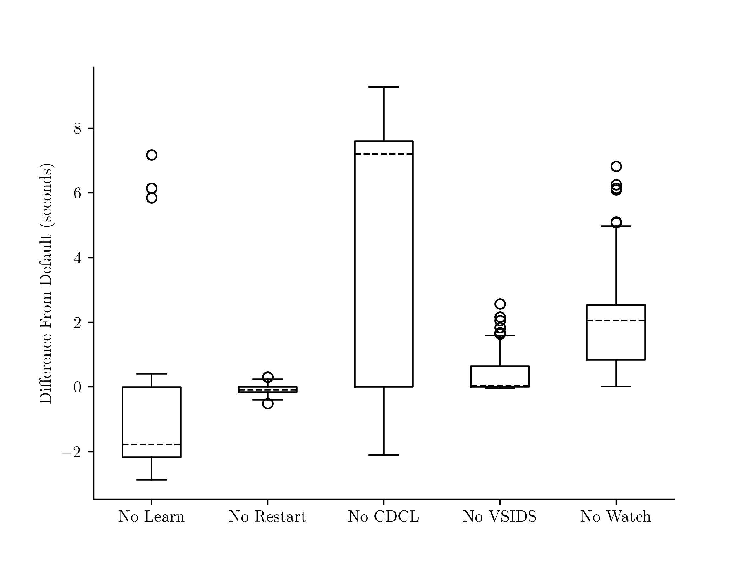
Figure 11. Performance synthesizing solutions to Survive--Steps on a width board across 1,000 random rule tuples for six SAT solver configurations relative to the default configuration. A negative value means the configuration was faster. From left to right, these correspond to the --no-learn, --no-restart, --no-cdcl, --no-vsids, and --no-watch configurations of the Biere's SATCH [43] solver.
We followed the approach of a previous empirical study [45] of SAT solver features. First, 1,000 tuples of elementary rules were sampled. For each tuple, we generated a CNF formula for Survive--Steps on a width board, then randomized the formula's clauses' contents and clause order ten times, giving ten semantically equivalent versions of each formula to average performance data over. We ran each SAT solver configuration on on all 10,000 formulas and took the average runtime across a tuple's randomized CNFs as the tuple's solve time.
This experiment investigated six SAT solver configurations, listed below. These are the same configurations tested by Katebi et. al. [45], chosen because they cover some of the most significant advances in SAT solving.
-
No Learn disables learned clauses, but keeps features like variable selection heuristics that use metadata from learned clauses.
-
No Restart stops the solver from periodically restarting the search. Restarts can be useful, for example, when the solver makes a poor decision early on causing it to explore a doomed part of the search space.
-
No CDCL disables all features related to learned clauses and uses the pure DPLL algorithm.
-
No VSIDS causes the solver to use the VMTF [7] variable selection heuristic instead of VSIDS [6].
-
No Watch disables the two-watched literals technique [6] for detecting unit propagation opportunities.
An illustration of the results is given by Figure 11, we ran each configuration with a ten-second timeout, and timed-out runs were given a value of ten seconds in the illustration. Interestingly, disabling clause learning consistently sped up synthesis, whereas the pure DPLL algorithm had high variance and frequently timed out. This suggests, that while the overhead from learned clauses slows down the solver, their metadata is useful.
7.3 Experiment 2
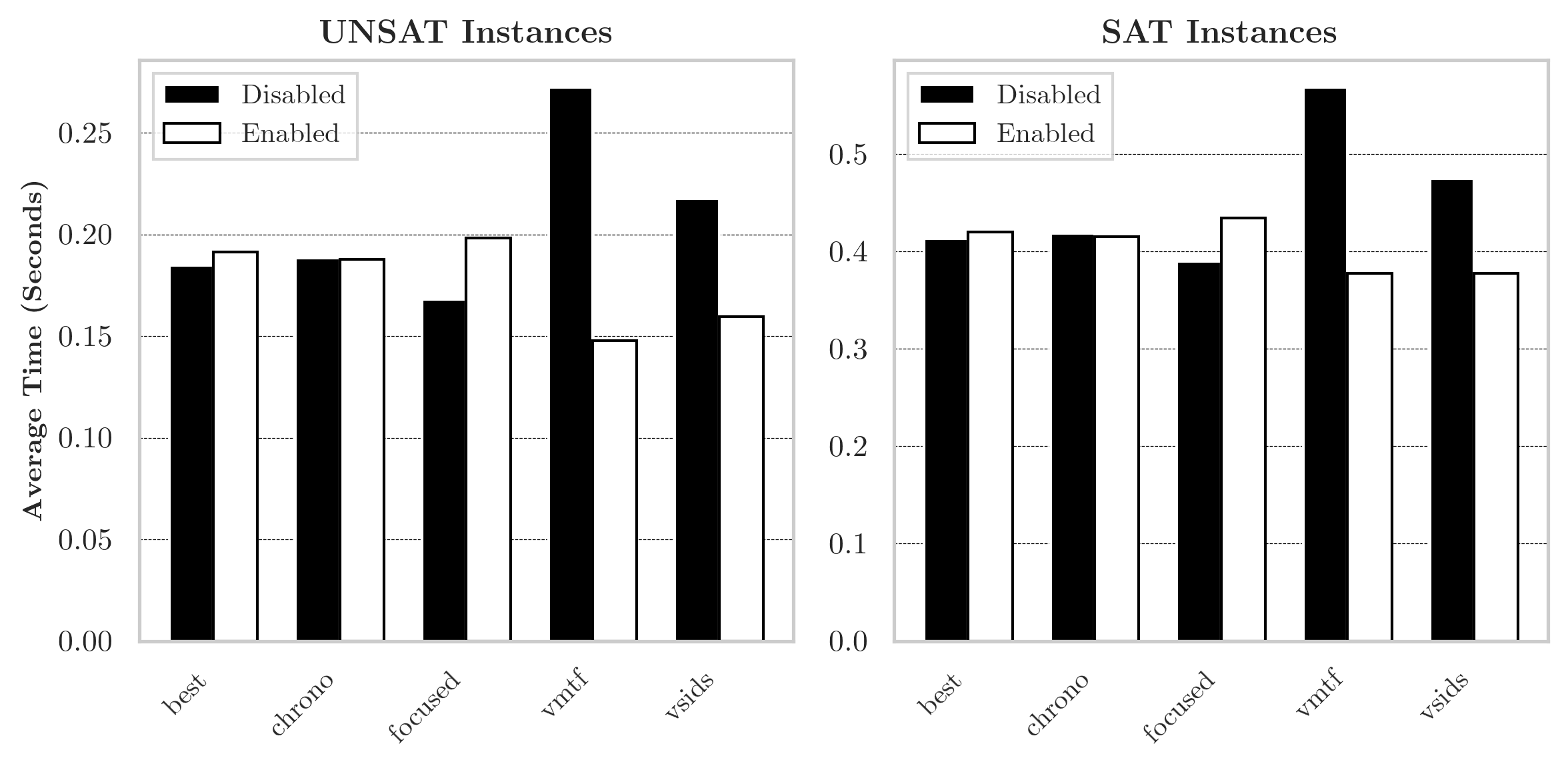
Figure 12. A comparison of the features disambiguating No Learn' and No CDCL' in Figure 11. For each permutation of features disambiguating the two, a solver was compiled and timed solving Survive--Steps for 1,000 random rule tuples on a width 31 board. The runtime above is the average across configurations where a feature is (en/dis)abled.
To better understand the difference between pure DPLL and the No Learn configurations, we repeated the experiment described in the first paragraph of §7.2 using SAT solvers configured with every permutation of the features which disambiguate pure DPLL and No Learn. Concretely, when the five configuration options listed below are disabled along with clause learning, the resulting configuration is equivalent to the pure DPLL configuration. For every way to (en/dis)able these five options along with No Learn we compiled a solver, and measured the performance of each solver using the method described in the first paragraph of §7.2. Then, for each feature, we took the average runtime on the randomly sampled CNF formulas for configurations it was (en/dis)abled in. The results are illustrated in Figure 12.
-
Best trail rephrasing, corresponds to the
–no-bestconfiguration option for SATCH. -
Chrono corresponds to non-chronological backtracking and the
–no-chronoconfiguration option. -
Focused (en/dis)ables focused mode [46] which causes the solver to alternate between periods of slow/rapid restarts. There is some empirical evidence [47] that periods of slow/rapid restarts are better for UNSAT/SAT formulas. Corresponds to the configuration option.
-
VMTF/VSIDS corresponds to variable selection heuristics as described in §7.2.
Of the features disambiguating pure DPLL and the No Learn configurations, variable selection heuristics had the largest impact. To understand this, we generated heatmaps of the frequency variables were selected using the VSIDS heuristic for a small, random selection of rule tuples. Three interesting examples are shown in Figure 13 alongside a visualization of a random assignment to the rule array. These examples, together with the effectiveness of variable selection heuristics shown in Figure 12, suggest there may be structural properties of the automata that are exploited by variable selection heuristics. More analysis of this could be interesting for future work.
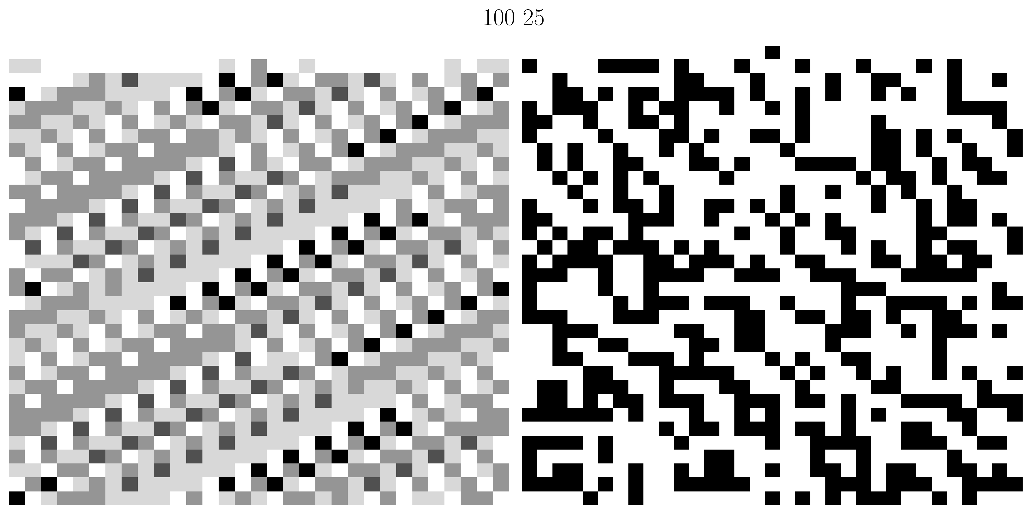
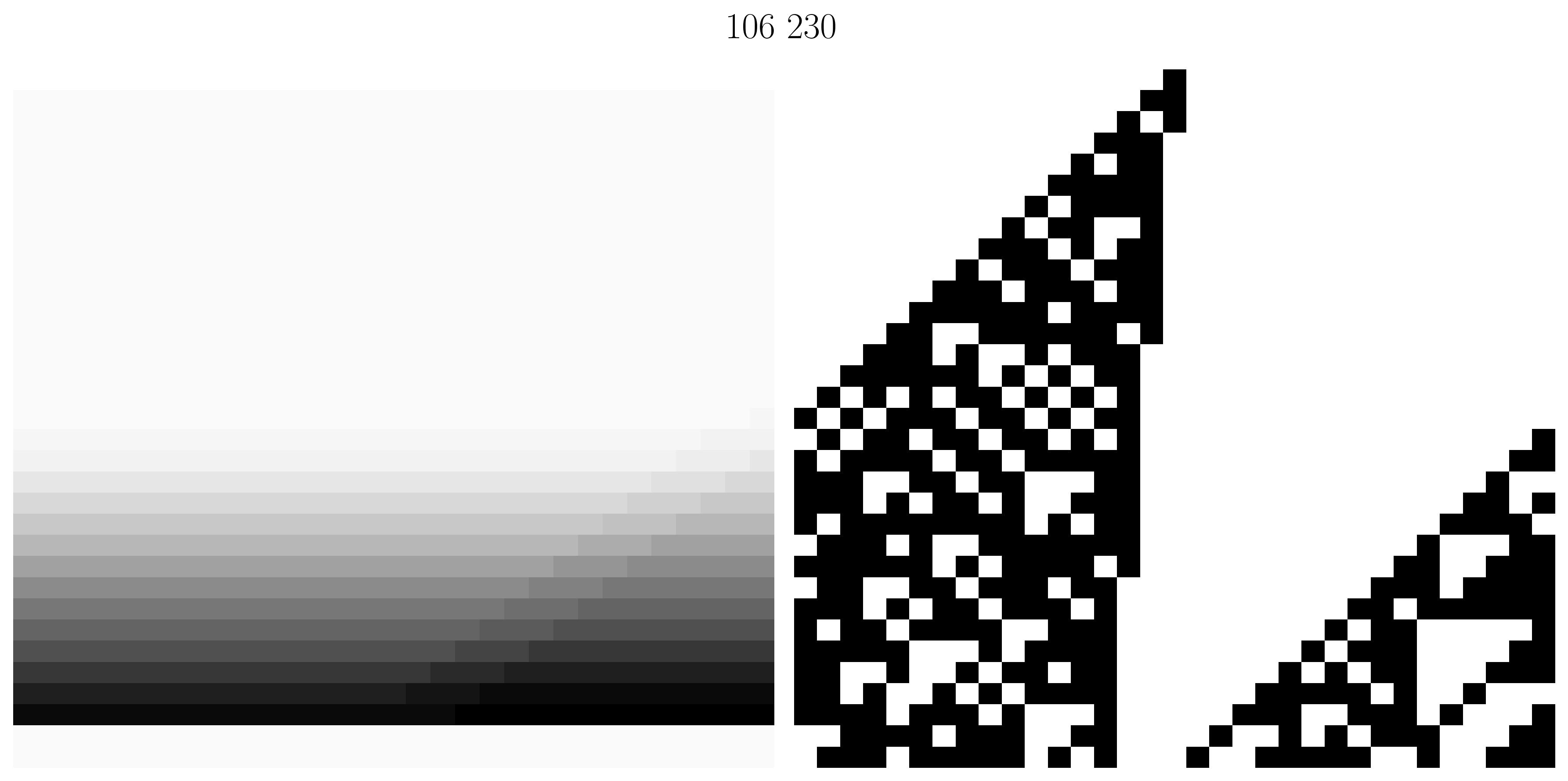
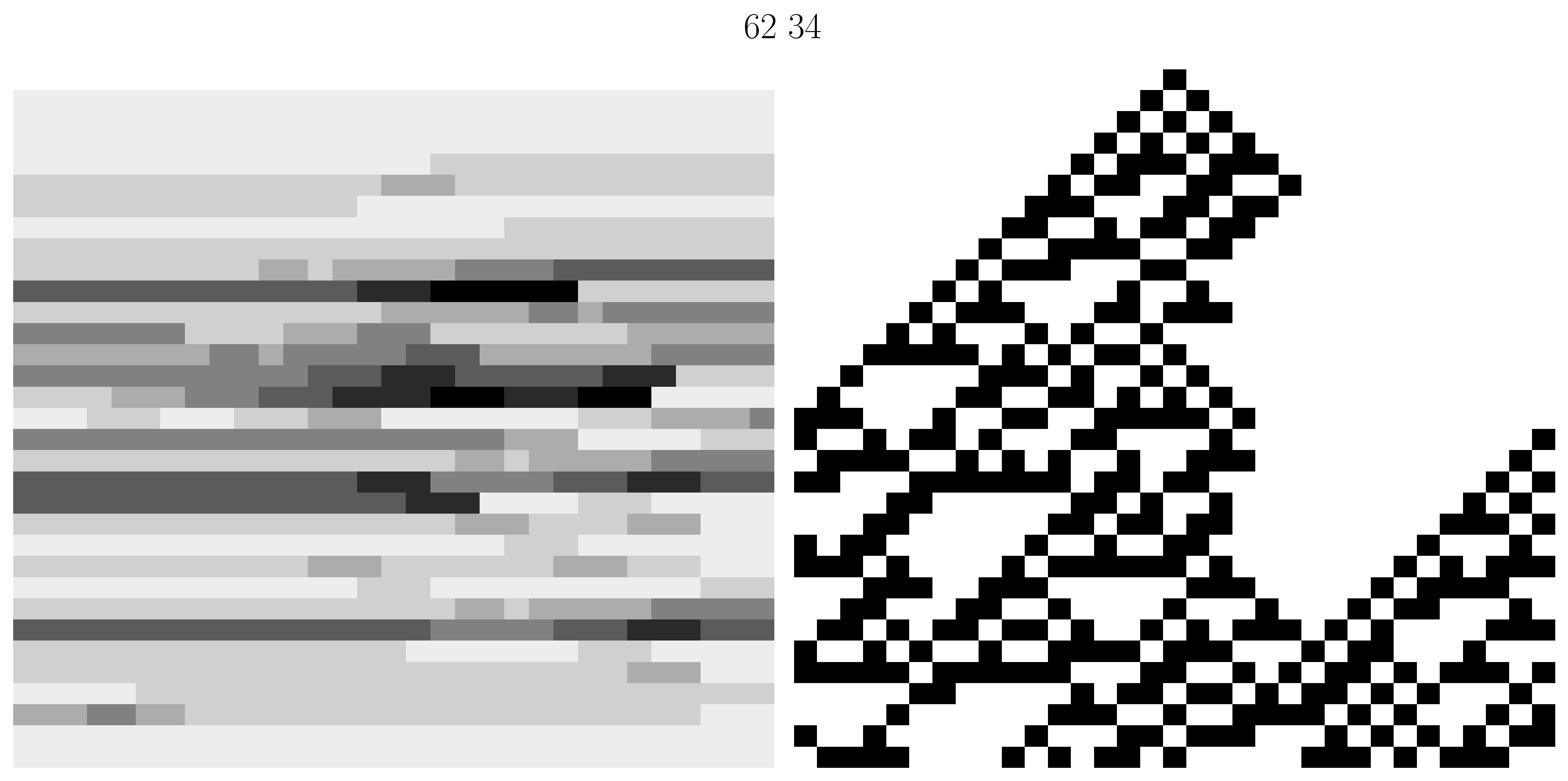
Figure 13. Three rule tuples. (Left Column) Heatmap of the frequency variables are selected using the VSIDS [6] variable selection heuristic while synthesizing a solution to Survive--Steps on a width board. A darker value at row column means was more frequently a decision variable. (Right Column) An inhomogeneous automaton using the rule tuple with a randomly initialized rule array. Visual similarities suggest VMTF could be exploring interesting properties of the automata.
8 Conclusion
Wolfram proposed the Survive--Steps problem and explored its connections to biology and neural networks. We gave novel methods for synthesizing and analyzing inhomogeneous cellular automata using Boolean satisfiability and BDDs and analyzed the problem. First, we exhaustively characterized what tuples of elementary cellular automata could be composed to survive steps on a width-31 board for . Then, we introduced several analytical and computational techniques to determine if the set of solvable is finite or infinite, demonstrating significant underlying structure within the problem. Finally, we studied what heuristics drive SAT solver performance, finding learned clauses are not effective, but variable selection heuristics are. Our work provides new analysis techniques for inhomogeneous cellular automata and suggests avenues for future work such as investigating the structure in our computational techniques to derive analytical versions (c.f. Figure 8), looking for theoretical insights that explain the effectiveness of variable selection heuristics, and extending our results on SAT solver performance to new synthesis algorithms and cellular automata classes.
Code Availability
Data and code to reproduce the experiments and figures in this post is available at: https://git.sr.ht/~ekez/survive-k/
Appendix A. Extended Proofs
A.1 Lemma 1
Proof. For with exactly one , Let and . We'll show that because solves Survive--Steps, , so solves Survive--Steps.
When this is trivially the case. When we'll proceed by induction using as our base case. Note that when , as solves Survive--Steps, so for our inductive hypothesis we get .
Notes
- With Lemma 3, it is relatively straightforward to prove that when is odd, rules 114 and 119 can only survive steps for . The basic idea being, at this height, on odd-width boards, due to the similarity of rules 114 and 119, wrapping forces
 to occur.
 - Notice, the omission of (9) leaves the initial state unconstrained.
- Obviously, when constructing this is intractable, so we use the logically-equivalent
existmethod provided bytulip-control/dd[42].
References
- What's Really Going On in Machine Learning? Some Minimal Models. Wolfram, Stephen. Stephen Wolfram Writings. 2024.
- Inhomogeneous Cellular Automata (INCA). Hartman, H. and Vichniac, G. Y.. Disordered Systems and Biological Organization. 1986.
- Why Does Biological Evolution Work? A Minimal Model for Biological Evolution and Other Adaptive Processes. Wolfram, Stephen. Stephen Wolfram Writings. 2024.
- Foundations of Biological Evolution: More Results & More Surprises. Wolfram, Stephen. Stephen Wolfram Writings. 2024.
- A machine program for theorem-proving. Davis, Martin, Logemann, George, Loveland, Donald. Communications of the ACM. 1962.
- Chaff: Engineering an Efficient SAT Solver. Matthew W. Moskewicz and Conor F. Madigan and Ying Zhao and Lintao Zhang and Sharad Malik. Proceedings of the 38th Design Automation Conference, DAC 2001, Las Vegas, NV, USA, June 18-22, 2001. 2001.
- Efficient algorithms for clause-learning SAT solvers. L. Ryan. 2004.
- On the generation of high-quality random numbers by two-dimensional cellular automata. Tomassini, M., Sipper, M., Perrenoud, M.. IEEE Transactions on Computers. 2000.
- Inhomogeneous cellular automata modeling for mixed traffic with cars and motorcycles. Lan, Lawrence W., Chang, Chiung-Wen. Journal of Advanced Transportation. 2005.
- Cellular automaton public-key cryptosystem. Rio Piedras, PR. Complex Systems. 1987.
- A survey of cellular automata: types, dynamics, non-uniformity and applications. Bhattacharjee, Kamalika, Naskar, Nazma, Roy, Souvik, Das, Sukanta. Natural Computing. 2020.
- Time-Reversal in Conway's Life as SAT. Stuart Bain. AI 2007: Advances in Artificial Intelligence, 20th Australian Joint Conference on Artificial Intelligence, Gold Coast, Australia, December 2-6, 2007, Proceedings. 2007.
- Mathematical Games: The fantastic combinations of John Conway's new solitaire game. Gardner, Martin. Scientific American. 1970.
- Compositional Object Synthesis in Game of Life Cellular Automata Using SAT Solver. Nishimura, Haruki, Hasebe, Koji. Advances in Swarm Intelligence: 12th International Conference, ICSI 2021, Qingdao, China, July 17–21, 2021, Proceedings, Part II. 2021.
- SAT-Based Analysis of Cellular Automata. Massimo D'Antonio and Giorgio Delzanno. Cellular Automata, 6th International Conference on Cellular Automata for Research and Industry, ACRI 2004, Amsterdam, The Netherlands, October 25-28, 2004, Proceedings. 2004.
- A Six-State Minimal Time Solution to the Firing Squad Synchronization Problem. Jacques Mazoyer. Theor. Comput. Sci.. 1987.
- Remarks on the cellular automaton global synchronisation problem: deterministic versus stochastic models. Fates, Nazim. Natural Computing. 2019.
- Discovery by Genetic Programming of a Cellular Automata Rule that is Better than any Known Rule for the Majority Classification Problem. David Andre, Forrest H. Bennett III, John R. Koza. Genetic Programming 1996: Proceedings of the First Annual Conference, July 28-31, 1996, Stanford University. 1996.
- Research of Complex Forms in Cellular Automata by Evolutionary Algorithms. Sapin, Emmanuel and Bailleux, Olivier and Chabrier, Jean-Jacques. Artificial Evolution. 2004.
- Synthesis of Desired Binary Cellular Automata Through the Genetic Algorithm. Suzuki, Satoshi and Saito, Toshimichi. Neural Information Processing. 2006.
- Evolving Cellular Automata. Cenek, Martin and Mitchell, Melanie. Computational Complexity: Theory, Techniques, and Applications. 2012.
- Evolving S-boxes based on cellular automata with genetic programming. Picek, Stjepan, Mariot, Luca, Leporati, Alberto, Jakobovic, Domagoj. Proceedings of the Genetic and Evolutionary Computation Conference Companion. 2017.
- Evolutionary algorithms for designing reversible cellular automata. Mariot, Luca, Picek, Stjepan, Jakobovic, Domagoj, Leporati, Alberto. Genetic Programming and Evolvable Machines. 2021.
- Co-evolving non-uniform cellular automata to perform computations. Moshe Sipper. Physica D: Nonlinear Phenomena. 1996.
- Evolving Cellular Automata to Perform User-Defined Computations. Grouchy, Paul, D'Eleuterio, Gabriele M.T.. 2016.
- Thread: Differentiable Self-organizing Systems. Mordvintsev, Alexander, Randazzo, Ettore, Niklasson, Eyvind, Levin, Michael, Greydanus, Sam. Distill. 2020.
- Differentiable Logic CA: from Game of Life to Pattern Generation. Pietro Miotti, Eyvind Niklasson, Ettore Randazzo, Alexander Mordvintsev. Paradigms of Intelligence. 2025.
- RC2: an Efficient MaxSAT Solver. Alexey Ignatiev and Antonio Morgado and Joao Marques-Silva. J. Satisf. Boolean Model. Comput.. 2019.
- Program Synthesis. Sumit Gulwani, Oleksandr Polozov, Rishabh Singh. Foundations and Trends® in Programming Languages. 2017.
- Syntax-Guided Synthesis. Rajeev Alur and Rastislav Bodik and Eric Dallal and Dana Fisman and Pranav Garg and Garvit Juniwal and Hadas Kress-Gazit and P. Madhusudan and Milo M. K. Martin and Mukund Raghothaman and Shambwaditya Saha and Sanjit A. Seshia and Rishabh Singh and Armando Solar-Lezama and Emina Torlak and Abhishek Udupa. Dependable Software Systems Engineering. 2015.
- Cellular Automata Surviving Steps. Zeke Medley and Panagiotis Manolios. Proceedings of the 19th International Workshop on the ACL2 Theorem Prover and Its Applications, Austin, TX, USA and online, May 12-13, 2025. 2025.
- ACL2s: "The ACL2 Sedan". Peter C. Dillinger, Panagiotis Manolios, Daron Vroon, J. Strother Moore. Proceedings of the 7th Workshop on User Interfaces for Theorem Provers (UITP 2006). 2007.
- A New Kind of Science. Wolfram, Stephen. 2002.
- On the Complexity of Derivation in Propositional Calculus. Tseitin, G. S.. Automation of Reasoning. 1968.
- PySAT: A Python Toolkit for Prototyping with SAT Oracles. Alexey Ignatiev and Antonio Morgado and Joao Marques-Silva. Theory and Applications of Satisfiability Testing - SAT 2018 - 21st International Conference, SAT 2018, Held as Part of the Federated Logic Conference, FloC 2018, Oxford, UK, July 9-12, 2018, Proceedings. 2018.
- Universality in Elementary Cellular Automata. Matthew Cook. Complex Syst.. 2004.
- On Patterns and Dynamics of Rule 22 Cellular Automaton. Genaro J. Martinez and Andrew Adamatzky and Rolf Hoffmann and Dominique Deserable and Ivan Zelinka. Complex Syst.. 2019.
- A Combinatorial Problem. De Bruijn, N. G.. Proceedings of the Koninklijke Nederlandse Akademie van Wetenschappen. 1946.
- Finding and counting given length cycles. Noga Alon, Raphael Yuster, Uri Zwick. Algorithmica. 1997.
- Towards an Optimal CNF Encoding of Boolean Cardinality Constraints. Carsten Sinz. Principles and Practice of Constraint Programming -- CP 2005. 2005.
- Coin Problem. Weisstein, Eric W.. From MathWorld--A Wolfram Web Resource.
- dd: Binary Decision Diagrams in pure Python and Cython wrappers of CUDD, Sylvan, and BuDDy. Filippidis, Ioannis, Haesaert, Sofie, Livingston, Scott C., Wenzel, Mario. Accessed: 2025-03-25. 2025.
- CNF Encodings of Complete Pairwise Combinatorial Testing of our SAT Solver Satch. Armin Biere. Proc. of SAT Competition 2021 -- Solver and Benchmark Descriptions. 2021.
- Conflict-Driven Clause Learning SAT Solvers. Joao Marques-Silva and Ines Lynce and Sharad Malik. Handbook of Satisfiability - Second Edition. 2021.
- Empirical Study of the Anatomy of Modern Sat Solvers. Hadi Katebi and Karem A. Sakallah and Joao P. Marques Silva. Theory and Applications of Satisfiability Testing - SAT 2011 - 14th International Conference, SAT 2011, Ann Arbor, MI, USA, June 19-22, 2011. Proceedings. 2011.
- Cadical, kissat, paracooba, plingeling and treengeling entering the sat competition 2020. Fleury, ABKFM, Heisinger, Maximilian. SAT COMPETITION. 2020.
- Between SAT and UNSAT: The Fundamental Difference in CDCL SAT. Chanseok Oh. Theory and Applications of Satisfiability Testing - SAT 2015 - 18th International Conference, Austin, TX, USA, September 24-27, 2015, Proceedings. 2015.
- The Silent (R)evolution of SAT. Johannes K. Fichte, Daniel Le Berre, Markus Hecher, Stefan Szeider. Communications of the ACM. 2023.
- GRASP: a search algorithm for propositional satisfiability. Marques-Silva, J.P., Sakallah, K.A.. IEEE Transactions on Computers. 1999.